See python code:https://github.com/felipeOL10/Corporate-credit-ratings-analysis

Data:https://www.kaggle.com/datasets/kirtandelwadia/corporate-credit-rating-with-financial-ratios

Goal of the project

• Analyse the determinants of investable corporate bonds;

• Using a logistic regression to predict the investible rating.

Data

Corporate credit ratings, issued by specialist agencies, provide an assessment about the credit worthiness of a company and acts as a pivotal financial indication to potential investors. It helps provide investors with a concrete idea about the risk associated with the company’s credit investment returns. Every company aims to attain a good credit rating for seeking more investment and lower debt interest rates.

Most of the credit rating agencies have a unique discrete ordinal rating scale. The rating scale of the S&P is: {AAA, AA+, AA, AA−, A+, A, A−, BBB+, BBB, BBB−, BB+, BB, BB−, B+, B, B−, CCC+, CCC, CCC−, CC, C, D} – a total of 22 grades that are ordered from AAA, the most promising one to D, the most risky one. S&P broadly classifies the companies with rating higher than BB+ as investment grade companies and others as junk grade companies. Credit ratings are mostly determined by financial ratios coming from balance sheets, income statements, and cash-flow statements.

Therefor, the dataset has 7805 rows with 25 columns, ranging from 2010 to 2016. The data incorporates several financial ratios and the corporate ratings.

list(corp_credit_rating.columns)

['Rating Agency', 'Corporation', 'Rating', 'Rating Date', 'CIK', 'Binary Rating', 'SIC Code', 'Sector', 'Ticker', 'Current Ratio', 'Long-term Debt / Capital', 'Debt/Equity Ratio', 'Gross Margin', 'Operating Margin', 'EBIT Margin', 'EBITDA Margin', 'Pre-Tax Profit Margin', 'Net Profit Margin', 'Asset Turnover', 'ROE - Return On Equity', 'Return On Tangible Equity', 'ROA - Return On Assets', 'ROI - Return On Investment', 'Operating Cash Flow Per Share', 'Free Cash Flow Per Share']

EDA

# Companies in dataset

corp_credit_rating.Corporation.unique()

array(['American States Water Co.', 'Automatic Data Processing Inc.', 'Avnet Inc.', ..., 'Xerox Corp.', 'YPF Sociedad Anonima', 'iHeartCommunications Inc.'], dtype=object)

# Sector in dataset

corp_credit_rating.Sector.unique()

Output array(['Utils', 'BusEq', 'Shops', 'Manuf', 'NoDur', 'Other', 'Chems', 'Telcm', 'Hlth', 'Money', 'Durbl', 'Enrgy'], dtype=object)

# Types of bonds in dataset

corp_credit_rating.Rating.unique()

array(['A-', 'AAA', 'BBB-', 'AA-', 'A', 'BBB+', 'BBB', 'BB', 'B', 'BB+', 'B+', 'BB-', 'B-', 'A+', 'CCC', 'AA', 'CCC+', 'CC', 'C', 'CCC-', 'AA+', 'D', 'CC+'], dtype=object)

# Check for missing values

corp_credit_rating[pd.isnull(corp_credit_rating)].count()

Rating Agency 0 Corporation 0 Rating 0 Rating Date 0 CIK 0 Binary Rating 0 SIC Code 0 Sector 0 Ticker 0 Current Ratio 0 Long-term Debt / Capital 0 Debt/Equity Ratio 0 Gross Margin 0 Operating Margin 0 EBIT Margin 0 EBITDA Margin 0 Pre-Tax Profit Margin 0 Net Profit Margin 0 Asset Turnover 0 ROE - Return On Equity 0 Return On Tangible Equity 0 ROA - Return On Assets 0 ROI - Return On Investment 0 Operating Cash Flow Per Share 0 Free Cash Flow Per Share 0 Date 0 dtype: int64

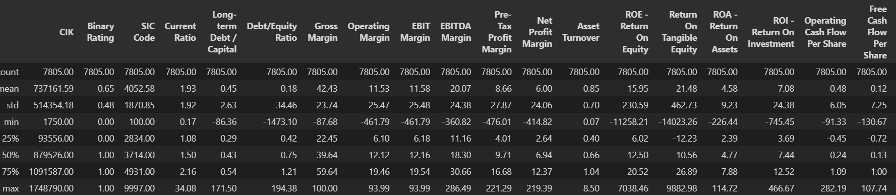
- The average long term debt/capital is 0.45

-Debt/Equity ratio is 0.18 on average, suggesting that there is low risk when looking at all sectors.

-The operating margins is, on average, 11.5%.

-The ROA and ROI are lower than 10%, however the return on tangeble equti is more than double of ROI.

-The companies in the dataset have CF to pay debt and/or dividents, suggested by positive FCF per share.

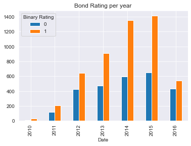
Good corporate credit ratings were the leading rating in all years analysed.

Till 2015 there was a significant growth of good ratings. In fact, this reflects the better economic outlook after the 2008 crises.

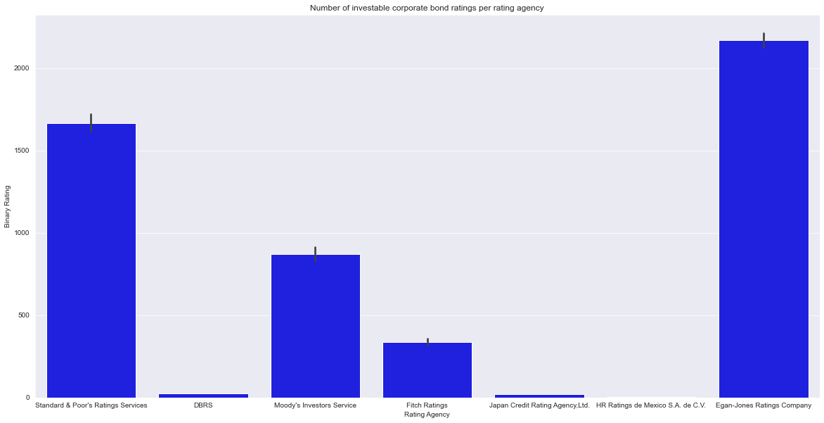
Egan-Jones were the leading agency to give good ratings with more than 2000 ratings.

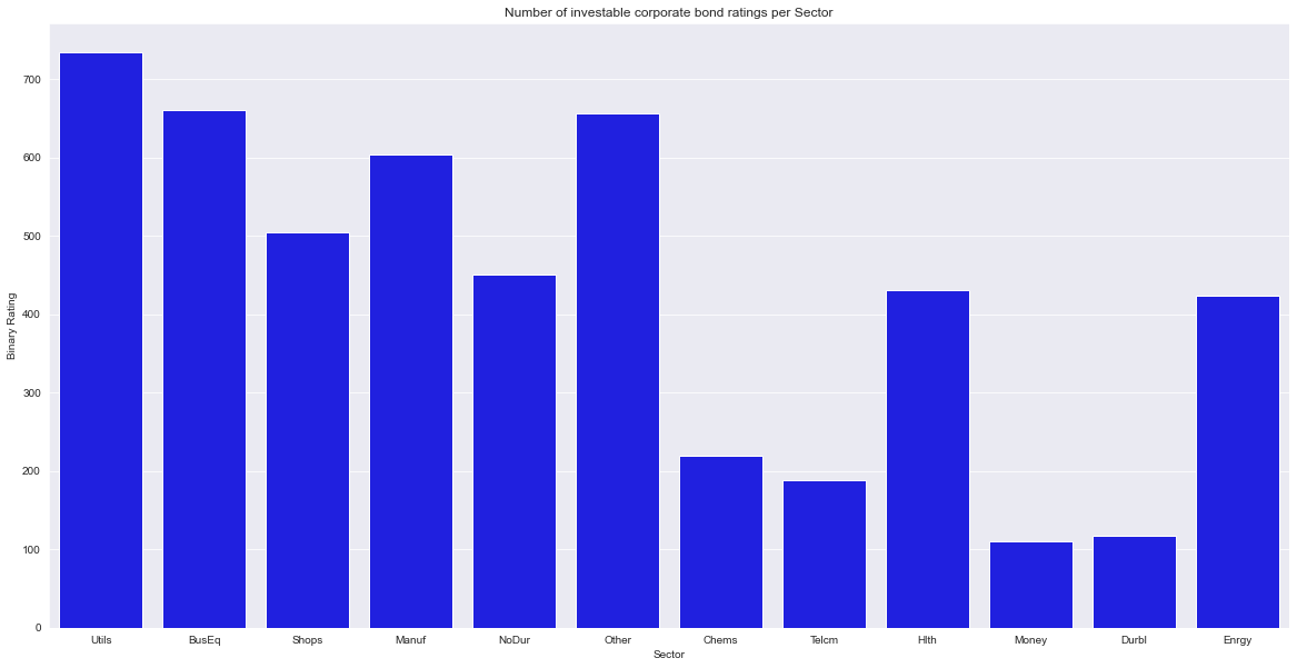
The utilities sector was the leading sector for good corporate credit ratings with more than 700.

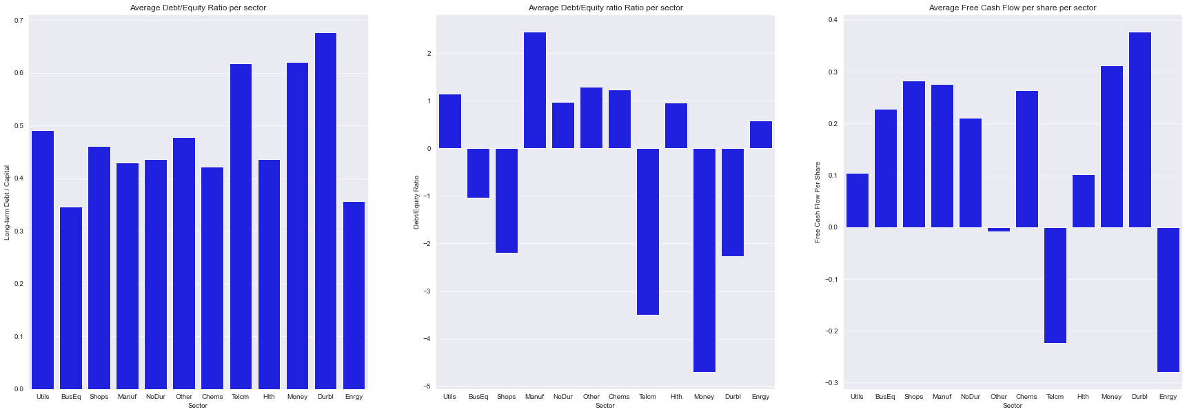
The debt-to-capital ratio is a measurement of a company's financial leverage, in this case, relative to long term-debt. Therefore, the "Durbl" category is the one with the highest ratio suggesting higher risk and possible lower credit rating. In fact, the last bar plot suggest that, in fact, this category is one of the lowest in terms of quality ratings. Moreover, the same case can be seen in the "money" and "telecom" category.

Generally, a good debt-to-equity ratio is considered lower than 1.0, a ratio of 2.0 or higher is usually considered risky. If a debt-to-equity ratio is negative, it means that the company has more liabilities than assets, thus extremely risky. Therefore, we can see that these sectors present all negative ratios, adding to the riskiness of the investment.

FCF per share signals the ability to pay debt. Therefore, the "Durbl" and money sectors presents good ability to pay debt. However, the energy, telecom and others suggest negative ratios, meaning they, in average, are not able to generate sufficient cash to support the business, thus suggesting higher risk.

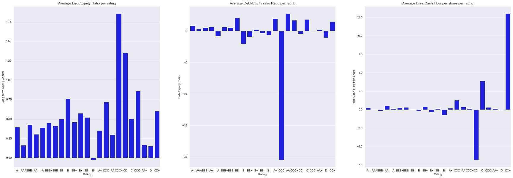
This bar plot suggest that good credit ratings are associeted with debt/capital ratios below 1, suggesting that this may be a good predictor. However, there is bad credit ratings that also are associeted with lower ratios, such as the D rating.

In terms of debt/equity, good credit ratings are associeted with positive and lower than 1 values, although there are some exceptions. In the other hand, bad credit ratings have generally negative ratios.

The FCF per share also suggest the same ideas as the other ratios, where good ratings, in general, have positive values.

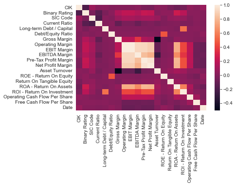
There is a high correlation between the binary rating, margin rations and ROA, suggesting that good margins and good financial performance move in the same direction.

There is a high correlation between ROI and long term debt/capita, ROE and gross margin and ROA and margin ratios. Therefore, having debt can be beneficial for better performance in terms of ROI and margins and performance move in the same direction, which is expected.

Logistic Regression

A logistic regression is a Machine Learning classification algorithm that is used to predict the probability of a categorical dependent variable. In logistic regression, the dependent variable is a binary variable that contains data coded as 1 (yes) or 0 (no). The classification goal is to predict whether the rating agency will give a investable rating to corporation.

SMOTE

One approach to addressing imbalanced datasets is to oversample the minority class. The simplest approach involves duplicating examples in the minority class, although these examples don’t add any new information to the model. Instead, new examples can be synthesized from the existing examples. This is a type of data augmentation for the minority class and is referred to as the Synthetic Minority Oversampling Technique, or SMOTE.

# Check if data is balanced

balance = data["Binary Rating"].value_counts()print(balance)

1 543 0 432 Name: Binary Rating, dtype: int64

There is an unbalance of the class zero.

os_data_X,os_data_y=os.fit_resample(X_train, y_train)

os_data_X = pd.DataFrame(data=os_data_X,columns=columns )

os_data_y= pd.DataFrame(data=os_data_y,columns=['Binary Rating'])

# we can Check the numbers of our data

print("length of oversampled data is ",len(os_data_X))

print("Number of non investable bonds in oversampled data",len(os_data_y[os_data_y['Binary Rating']==0]))

print("Number of investable bonds",len(os_data_y[os_data_y['Binary Rating']==1]))

print("Proportion of non investable bonds data in oversampled data is ",len(os_data_y[os_data_y['Binary Rating']==0])/len(os_data_X))

print("Proportion of investable bonds data in oversampled data is ",len(os_data_y[os_data_y['Binary Rating']==1])/len(os_data_X))

Output length of oversampled data is 778 Number of non investable bonds in oversampled data 389 Number of investable bonds 389 Proportion of non investable bonds data in oversampled data is 0.5 Proportion of investable bonds data in oversampled data is 0.5

# Check if data is balanced

balance = os_data_y.value_counts()

print(balance)

Binary Rating 0 389 1 389 dtype: int64


RFE

RFE is based on the idea to repeatedly construct a model and choose either the best or worst performing feature, setting the feature aside and then repeating the process with the rest of the features. This process is applied until all features in the dataset are exhausted.

# Chossing variables

logreg = LogisticRegression()

rfe = RFE(logreg)

rfe = rfe.fit(X, y.values.ravel())

print(rfe.support_)

print(rfe.ranking_)

Output

[ True True False False True True False False True True False False False True False True] [1 1 6 4 1 1 2 5 1 1 8 9 3 1 7 1]

Therefore, the variables suited are: 'Current Ratio', 'Long-term Debt / Capital','Operating Margin', 'EBIT Margin','Net Profit Margin', 'Asset Turnover','ROI - Return On Investment','Free Cash Flow Per Share'

Regression

X = os_data_X[['Current Ratio', 'Long-term Debt / Capital','Operating Margin', 'EBIT Margin','Net Profit Margin', 'Asset Turnover','ROI - Return On Investment','Free Cash Flow Per Share']]

y = os_data_y

X = sm.add_constant(X)

X_train, X_test, y_train, y_test = train_test_split(X, y)

logit_model = sm.Logit(y,X)

result = logit_model.fit()

print(result.summary2())

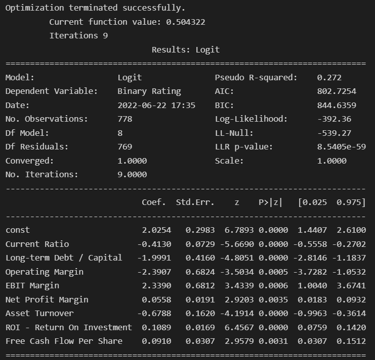
The model suggests that:

All variables selected are significant at 1%, and therefore can explain the binary rating.

Ebit margin, net profit margin, ROI and Free CF per share have all positive coeficients. Therefore, higher levels of all these ratios lead to higher probability of an investable rating, especially in the case of the ebit margin.

Current ratio, Long term Debt/Capital, Operating margin and asset turnover have all negative coeficients. Thus,higher levels of all these ratios lead to lower probability of an investable rating, especially in the case of operating margin.

y_pred = logreg.predict(X_test)

print('Accuracy of logistic regression classifier on test set: {:.2f}'.format(logreg.score(X_test, y_test)))

Accuracy of logistic regression classifier on test set: 0.79

Confusion matrix

from sklearn.metrics import confusion_matrix

confusion_matrix = confusion_matrix(y_test, y_pred)

print(confusion_matrix)

[[ 85 32] [ 17 100]]

This result sugests that 85+100 are correct predictions and 17+32 are incorrect predictions.

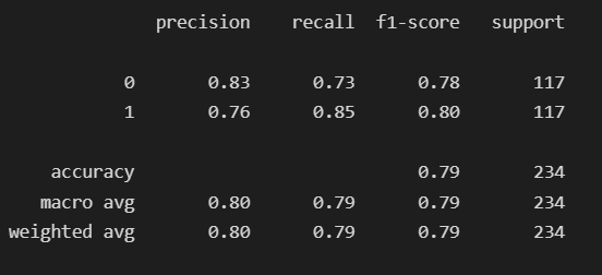
print(classification_report(y_test, y_pred))

To quote from Scikit Learn:

The precision is the ratio tp / (tp + fp) where tp is the number of true positives and fp the number of false positives. The precision is intuitively the ability of the classifier to not label a sample as positive if it is negative. Therefore, 80% of prediction were correct.

The recall is the ratio tp / (tp + fn) where tp is the number of true positives and fn the number of false negatives. The recall is intuitively the ability of the classifier to find all the positive samples. Thus, 79% of the investable rating were correctly identified.

The F-beta score can be interpreted as a weighted harmonic mean of the precision and recall, where an F-beta score reaches its best value at 1 and worst score at 0. Therefore, 79% of the positive prediction were correct.

The F-beta score weights the recall more than the precision by a factor of beta. beta = 1.0 means recall and precision are equally important.

The support is the number of occurrences of each class in y_test.

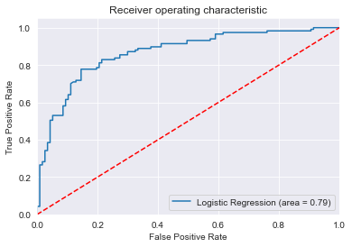
ROC

The ROC curve is another common tool used for this type of models. The dotted line represents the ROC curve of a purely random classifier; a good classifier stays as far away from that line as possible (toward the top-left corner).

Conclusion

Ebit margin, net profit margin, ROI, Free CF per share, current ratio, Long term Debt/Capital, Operating margin and asset turnover are all significant and determinants for the probability of having an investable rating.

Ebit margin, net profit margin, ROI and Free CF per share increses the probability of having an investable rating.

Current ratio, Long term Debt/Capital, Operating margin and asset turnover lower the probability of having an investable rating.

79% of the investable ratings were correct by the model.